Matlab Primer

Today's lecture will be on MATLAB and PENDULA (plural of PENDULUM). Your next lab assignment motivated the topic.

My name is Sean Carver; I am a research scientist in Mechanical Engineering. I have been programming in MATLAB for almost 20 years and programming computers for almost 30 years.

This class is about MATLAB, not about deriving equations. So I am just going to give you the equations for the PENDULUM. There is still a lot to do to get it into MATLAB.

Pendulum on a movable support

This example comes from Wikipedia (copied legally). Consider a pendulum of mass m and length ℓ, which is attached to a support with mass M which can move along a line in the x-direction. Let x be the coordinate along the line of the support, and let us denote the position of the pendulum by the angle θ from the vertical.

Sketch of the situation with definition of the coordinates (click to enlarge)

$\ddot\theta + \frac{\ddot x}{\ell} \cos\theta + \frac{g}{\ell} \sin\theta = 0.\,$

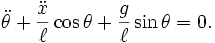
See http://en.wikipedia.org/w/index.php?title=Lagrangian_mechanics&oldid=516894618 for a full derivation.

Challenge (not required): implement this model, after seeing how to implement a simpler one, below.

Pendulum on a fixed support

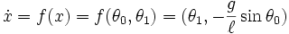
Together we are going to implement a simpler model with a fixed and unmovable support. You can easily see how to modify the above equations. Just plug in

$\ddot x = \dot x = x = 0$

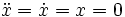
The second term drops out:

$\ddot\theta + \frac{g}{\ell} \sin\theta = 0.\,$

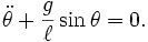
Step 1: Make the model first order (first derivatives only)

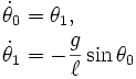
Define new variables

$\begin{align} \theta_0 & = \theta, \\ \theta_1 & = \dot\theta \end{align}$

Now we have two equations:

$\begin{align} \dot\theta_0 & = \theta_1, \\ \dot\theta_1 & = - \frac{g}{\ell} \sin\theta_0 \end{align}$

Step 2: Discretize the model

This is a tricky step. Choices must be made. There are many many methods for discretizing a differential equation. There about a dozen MATLAB routines that will do it for you... but then you have to learn how to use them. We will write our own routine implementing the very simplest method...Euler's method.

Euler's Method:

Write the first order variables of the differential equation as a vector:

$x = (\theta_0,\theta_1)$

Write the differential equation as a vector

$\dot x = f(x) = f(\theta_0,\theta_1) = (\theta_1, - \frac{g}{\ell} \sin\theta_0 )$

The set of possible values for the vector x is the called the phase space for the differential equation, and f(x) is the velocity of through the phase space.

Euler's method says the next point in phase space is equal to the current point plus the time step times the velocity.

Now Euler's method is given by the following recursion

$x_k = x_{k-1} + dt \ f(x_{k-1})$

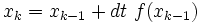
This get translated into the following MATLAB code

theta0(k) = theta0(k-1) + dt * theta1(k-1);
theta1(k) = theta1(k-1) - dt * (g/l)*sin(theta0(k-1));

The whole program

We are going to write a MATLAB "function" to simulate the pendulum. A function has the following form:

function [OutputArguments] = functionName(InputArguments)
% Help Comments

[Statements...All variables defined here will be forgotten once the function completes]

end 

A function is "called" with the command:

[OutputArguments] = functionName(InputArguments);

Our function looks like this

function [theta0,theta1,time] = pend(ang,vel,l,dt,tmax)
% Function to simulate pendulum
%  [theta0,theta1,time] = pend(ang,vel,l,dt,tmax)
%  INPUT: ang (intial angle), vel (initial velocity), l (length of pendulum)
%             dt (time step), tmax (final time)
%  OUTPUT: theta0 (trajectory of angle) 
%                theta1 (trajectory of angular velocity
%                 time (trajectory of time (for plotting)

g = 9.8;
time = dt:dt:tmax;
kmax = length(time);

% Need to initialize vectors; otherwise runs slowly
theta0 = zeros(1,kmax);
theta1 = zeros(1,kmax);

% Put in initial conditions
theta0(1) = ang;
theta1(1) = vel;

for k=2:kmax
   theta0(k) = theta0(k-1) + dt * theta1(k-1);
   theta1(k) = theta1(k-1) - dt * (g/l)*sin(theta0(k-1));
end
end

Copy and paste the above code into your MATLAB editor (if your editor is not visible, type "edit" into the command window, and press return). Once the you have copied the above function into the editor, save as pend.m.

Running the program and plotting results

To run the pendulum code, copy and paste the following commands into your MATLAB command window:

First define the variables to be passed to the function. Notice that the names here need not be the same as the ones used in the function.

InitialAngle = 5*pi/6;
InitialVelocity = 0;
len = 1;
dt = 0.0001;
stopTime = 10;

Now call the function

[theta0,theta1,time] = pend(InitialAngle,InitialVelocity,len,dt,stopTime);

Now plot the output:

figure(1)
plot(time,theta0,'b');
figure(2)
plot(time,theta1,'g');
figure(3)
plot(theta0,theta1,'r');

You can add axis labels to your plots. First bring the plot to the front then add the labels:

figure(3)
xlabel('Angle (radians)');
ylabel('Angular velocity (radians/sec)');

Now add the axis labels to the others. This is what you should see:

Time versus angle (click to enlarge)

Time versus angular velocity (click to enlarge)

Angle versus angular velocity (click to enlarge)

If you want to overlay two or more plots on the same axis:

plot(**First plot**)
hold on
plot(**Remaining Plots**)

Then if you want to erase:

hold off
plot(**New plot**)

Animating the Pendulum

Interpreting the above plots can be hard at first. What we would really like to do is see the pendulum move. I will show you how.

I have written a rather complicated function. Most of the complications were added in order to make things look good. Here is the code that animates the pendulum: (Copy and paste into a new function in the MATLAB editor, and save as animate_pendulum.m)

function animate_pendulum(AnimationSpeed,time,theta0,theta1)
% animate_pend -- Function to animate pendulum
% INPUT AnimationSpeed (try 1)
%       time,theta0,theta1 (output from simulation)
% OUTPUT: This function has no variable outputs (just animation)

FramesPerSecond = 30;
% wait is the length of time in seconds the animation waits between frames
wait = 1/FramesPerSecond;

% skip is the number of time steps of the simulation to skip
%      the following formula is my attempt to make real time equal
%      simulated time when speed = 1.
%       Doesn't work, animation too slow, but reasonable.
skip = round(AnimationSpeed/(FramesPerSecond*(time(2)-time(1))));

% Set figure.
figure(1);
set(gcf,'Renderer','OpenGL');

kmax = length(time);

% PENDULUM
% Plot pendulum
subplot(1,2,1);
hold off
Pshaft = plot([0,sin(theta0(1))],[0,-cos(theta0(1))],'r');
hold on
Panchor = plot(0,0,'r*');
Pmass = plot(sin(theta0(1)),-cos(theta0(1)),'ro');

% Change characteristics of Pendulum Plot
set(Panchor,'MarkerSize',20);
set(Panchor,'LineWidth',2);
set(Pshaft,'LineWidth',4);
set(Pmass,'MarkerSize',20);
set(Pmass,'LineWidth',4);
set(Pshaft,'EraseMode','normal');
set(Pmass,'EraseMode','normal')
axis equal
axis([-2,2,-2,2])
set(gca,'XTick',[]);
set(gca,'YTick',[]);
  
% PHASE PLOT
% Plot phase portrait
% For plotting purposes remap angles so that -pi <- angles < pi.
subplot(1,2,2);
hold off
Ptrajectory = plot(mod(theta0+pi,2*pi)-pi,theta1,'r.');
hold on
Pphasepoint = plot(mod(theta0(1)+pi,2*pi)-pi,theta1(1),'*');

% Change characteristics of phase plot
set(Pphasepoint,'MarkerSize',20);
set(Pphasepoint,'LineWidth',3);
set(Pphasepoint,'EraseMode','normal');
set(Ptrajectory,'MarkerSize',4);
axis([-pi,pi,-10,10]);
set(gca,'XTick',[-pi,-pi/2,0,pi/2,pi]);
set(gca,'XTickLabel',{'-pi','-pi/2','0','pi/2','pi'}) 
XL = xlabel('Angle (rad)'); 
YL = ylabel('Angular velocity (rad/s)');
set(XL,'FontWeight','Bold');
set(XL,'FontSize',17);
set(YL,'FontWeight','Bold');
set(YL,'FontSize',17);

% LOOP and animate
for k = 1:skip:kmax
  set(Pshaft,'XData',[0,sin(theta0(k))]);
  set(Pshaft,'YData',[0,-cos(theta0(k))]);
  set(Pmass,'XData',sin(theta0(k)));
  set(Pmass,'YData',-cos(theta0(k)));
  set(Pphasepoint,'XData',mod(theta0(k)+pi,2*pi)-pi); %-pi<=angles<pi
  set(Pphasepoint,'YData',theta1(k));
  pause(wait); 
end
end

Generate some data and define the new input parameter

[theta0,theta1,time] = pend(InitialAngle,InitialVelocity,len,dt,stopTime);
AnimationSpeed = 1;

Now animate the pendulum

animate_pendulum(AnimationSpeed,time,theta0,theta1);

Choosing Initial Angle & Initial Angular Velocity with the Mouse

After running an animation, run the following function:

function reanimate(len,dt,tmax,AnimationSpeed)
% Reanimate pendulum picking initial condition with mouse

% Make sure the focus is on the right figure and axis
figure(1);
subplot(1,2,2);
axis([-pi,pi,-10,10]);

% Command to input from the mouse
xy = ginput(1);

% Call functions to generate data and animate data
[theta0,theta1,time] = pend(xy(1),xy(2),len,dt,tmax);
animate_pendulum(AnimationSpeed,time,theta0,theta1);

end

Now call reanimate (animation window must still be on desktop). After calling reanimate, put the mouse somewhere over the rightmost axis, then press left mouse button.

reanimate(len,dt,stopTime,AnimationSpeed)

Questions

• Try InitialAngle=pi, InitialVelocity = 1. What is different about this trajectory?

• Try InitialAngle=pi, InitialVelocity = -1. What is different about this trajectory?

• What happens for small angles when (sin(theta0) = theta0)?

• We use a very small time step (input argument dt). Smaller time steps mean more accurate integration, but also more expensive computations. What happens when we increase the time step?

• Return to a small time step (re-execute the commands defining the input parameters). Verify that you are back by running another animation. Then consider a damped pendulum (pendulum with friction). The equation is below.

$\ddot\theta + \frac{g}{\ell} \sin\theta + b \dot\theta = 0.\,$

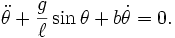
• Use "Save As" to create a new function, initially the same as pend.m. Call the new function damped_pend.m. This function has one more input parameter b, so add that to the parameter list then modify the function to add friction. You can use animate without any modification.

• Reanimate will need to be modified. "Save As" damped_reanimate.m then make the modification.

• Try with b = 0. This turns friction off. You should get same as without friction.

• Try with b = 1. What do you see?

• Try with b = 0.1. How does this differ?

• Try with b = -1. (Negative friction). What happens?