Bayesian Filtering

Here is the problem -- there is an open state (O) and closed state (C) and a stuck (inactivated) state (S). Transitions between these states happen like this

$O \rightleftharpoons C \rightleftharpoons S$

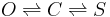
Transitions between O and S never happen (i.e. the probability is negligible) without C being an intermediary state. The observed current is zero in C and S and one in O. And there is noise. Transitions between C and S are invisible because there is no change in current. We want to estimate the transition probabilities. (The probabilities will depend upon the time step, but say the time step is fixed).

First generate some data which looks like.

Click image for full size

The transition probabilities for this plot are

Probability(Stay in Open) = 0.95
Probability(Open --> Closed) = 0.05
Probability(Open --> Stuck/Inactive) = 0.00

Probability(Closed --> Open) = 0.10
Probability(Stay in Closed) = 0.85
Probability(Closed --> Stuck) = 0.05

Probability(Stuck --> Open) = 0.00
Probability(Stuck -- Closed) = 0.003
Probability(Stay in Stuck) = 0.097

There are nine parameters here, but there is a constraint that each block add to 1, so we only have 6 parameter to estimate. Moreover we might know that transition between open and stuck never happen, so there would only be 4 parameters to estimate.

Thus the likelihood function is a function from four parameters to one value (likelihood). Too many to plot. Let's say we know the probabilities of going back and forth between open and closed. Thus we need only know the probabilities of going back and forth between closed and stuck (the invisible transitions).

We are going to compute the likelihood as we vary

P(Stuck --> Closed) from 0.001 to 0.010
P(Closed --> Stuck) from 0.01 to 0.12

Actually, the way I wrote the program it computes

P(Stuck --> Closed) from 0.001 to 0.010
P(Stay in Closed) from 0.01 to 0.12

The two are equivalent because P(Closed --> Open) is correctly known and the three "from Closed" probabilities add to 1.

Here are what it looks like:

Click image for full size

And with two different seeds:

Click image for full size

Click image for full size

I was concerned about the first plot, until I plotted the next two. Then I realized that the algorithm tries to estimate the probabilities of relatively rare events based on a limited amount of data (5000 data points). The performance may not look great at first sight, but consider how subtle are the inferences that it is trying to make. The estimates are reasonably close ... at least within the ballpark. It would look better zoomed out. With a lot more data, one can expect the estimates to be much better.

The purpose of the lecture is to present the Bayesian filtering algorithm.

Prerequisites

• You need to know (or guess) initial probabilities for each state, e.g say we know the channel starts open: P(Open) = 1, P(Closed) = 0, P(Stuck) = 0. In the code (linked below), I called P(Open), "Ostart," etc.

• You need transition probabilities. Lets say there are n states (i.e. three states, Open = 1, Closed = 2, Stuck = 3). Then p_ij is the probability of going to state j, assuming you start in state i.

• You need to know the probability density function for the data measurement given that you are in each state. For example, in the code, densities are Gaussian, the means are (1,0,0) for (open, closed, stuck) and the standard deviation for all is 0.01. In this case the means for open and closed/stuck are separated by 100 standard deviations -- you assume essentially no measurement noise.

• You need the data.

Step One: Start with Initial Probabilities for State And Make a Prediction for Next Time Step

Initial Probabilities

$P(X_0 = i)$

Predicted Probabilities

$P(X_1 = j) = \sum_i P(x_0 = i) p_{ij}$

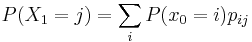
For example, the predicted probability that you are in CLOSED after the first time step (but before more information is gathered) is

• Probability that you start OPEN times probability that you transition from OPEN to CLOSED

• PLUS Probability that you start CLOSED times probability that you stay CLOSED

• PLUS Probability that you start STUCK times probability you transition from STUCK TO CLOSED

Same formula for the other states (OPEN AND STUCK).