MoreLikelihood
First of all thank you for completing the first survey. I have read and put a lot of thought into the responses. See the results here.
If you did not get my email (I did not have a complete list of addresses), click here.
Contents
Review
- Random number generators (rand and randn) produced differently distributed pseudo-random numbers.
- Setting the random seed allows you to reproduce the same random numbers.
>> randn('state',0)
>> randn

ans =

   -0.4326

>> randn

ans =

   -1.6656

>> randn

ans =

    0.1253

>> randn('state',0)
>> randn

ans =

   -0.4326

>> randn

ans =

   -1.6656

>> randn

ans =

   0.1253

>> randn('state',1)
>> randn

ans =

    0.8644

>> randn

ans =

    0.0942

>> randn

ans =

   -0.8519
- Remember the help and type and lookfor commands. These are three good commands to know for learning more about MATLAB which is beyond the scope of the class.
- Statistics: mean, median, mode, std, min, max. These MATLAB commands are functions of data, but they have theoretical counterparts which depend upon the PMF or PDF.
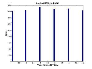
- For discrete random variables: Probability Mass Function which is the function of the possible values of random variable equal to the fraction of throws that land on the value. Remember the histogram for the dice experiment.
Remember that the histogram plots count (approximately 1/6 times number of throws) against value (1,2,3,4,5 or 6) where as the PMF plots limiting fraction (exactly 1/6) against value (1,2,3,4,5, or 6).
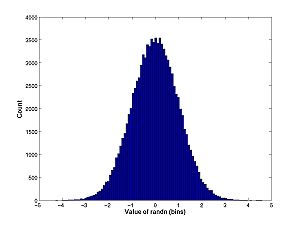
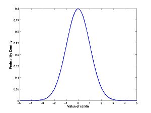
- For continuous random variables: Probability Density Function which is the function of the possible values of the random variable equal to the fraction of throws that land in a bin divided by width of bin, or actually the limit of this fraction as the bin width (bin containing the value) converges to 0.
Compare the histogram:
With the PDF:
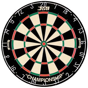
- Not review but extension: The axiomatic theory of probability always has in mind a set of outcomes of the experiment at hand. A random variable is a "real valued" function of the possible outcomes of the experiment. The possible values of the random variable might be the same as the possible outcomes, or there might be more outcomes. Example: Say the experiment is to throw a dart at a dartboard and the random variable is the number of points awarded. The values of the random variable are the integers between 0 and 100. The possible outcomes of the experiment could be the number of points awarded or it could be the (Cartesian or polar) coordinates of the dart on the board. In the latter case, infinitely many outcomes yeild the same value of the random variable.
- Following up the last 3 points, the PMF and PDF are always functions mapping all real numbers to probabilites (between 1 and 0) or probability densities (between 0 and infinity).
- Functions of random variables lead to new random variables. This allows more possibilities than rand and randn. Also note that these functions of rand and randn can depend on other quantities (parameters).
Some values returned by composing rand with a sigmoid function from last lab:
0.9611
0.0176
0.9818
0.9269
0.9550
0.0153
0.9515
0.0321
0.9124
0.1922
0.1460
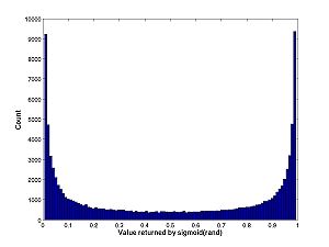
Note that values tend to either be close to 0 or close to 1 but not close to 0.5. You can see this property with the histogram:
- The likelihood function is the probability density as a function of parameters, ususally when the outcome of the experiment has already been observed.
- This likelihood function (for only one data point/dart throw) is not very useful. It becomes more useful when we consider many data throws. Let's start with two.
Homework from Lab B
Completed homework from Lab B is here.
People had difficulty with problem 5. Recall the instuctions:
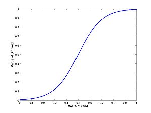
Now let's try it with the sigmoid function. First plot it:
A = 0:0.01:1;
F = sigmoid(A,.1,0.5);
plot(A,F);
Now
A = rand(10000,1);
F = sigmoid(A,.1,0.5);
hist(F,100)
- Homework B.5 (from Lab B): Consider the uniform random variable A = rand and the random variable F = sigmoid(A,k,h). Where does the PDF of F have peaks; where does it have troughs. Hint: For different k,h, be sure to plot both the function over the range of rand (0 to 1) and the histogram.
Many students did not execute the commands in order. If I had anticipated this I would have used different names (A and B) instead of just A. Your plots for problem 5 should have looked like this:
And
Problem 5 would have been very hard if the plots were not right.
Here is a sampling of students bonus problems.
Two Random Variables, Independence
Consider two examples of two random variables:
- Two calls to randn (or two throws of the dice).
- The membrane potential of a cell under study at 12:00 noon, yesterday, and the membrane potential of the same cell 10 microseconds later.
See the difference? In the first case, the value of the first random variable tells you nothing about the value of the second. In the second case, if you measure the membrane potential at 12:00 noon to be -60 mV, you can be quite sure that ten microseconds later that the membrane potential is close to (but not necessarily exactly) -60 mV. The point is, if you didn't know the value at 12:00 noon, you would be much less certain about the second value.
If the value of one random variable tells you nothing about the value of the other, we say the random variables are independent.
What does this mean mathematically? The mathematical definition of independence is written in terms of certain densities. There are three types of densities for two random variables X1, X2.
- Marginal densities: p(X1), p(X2).
- Joint density: p(X1,X2).
- Conditional densities p(X1|X2) and p(X2|X1).
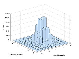
The difference is best described with a picture. First generate some data:
A = randn(100000,2)
This repeats the experiment 100000 times of calling randn twice. If you have access to the Statistics Toolbox (you don't on the machines in the classroom) you generate the plot below with this command:
hist3(A)
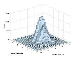
This is what you would see:
This is OK, but more resolution (more bins) is better. Try 30 x 30 bins:
hist3(A,[30,30])
If you don't have the Statistics toolbox, download the free version, hist2d here. Now type
hist2d(A)
I think this will work, but if it does not, you need to put the downloaded file in a place where matlab will see it. To see what MATLAB's current directory is, type
pwd
then move the file to that directory. I do not think this will be necessary in the classroom (I tried it already), but if it is necessary, there may be problems with permissions to write to MATLAB's current directory. Get help from me if this is the case.
What are we looking at: rows of bins correspond to the first call of randn and columns correspond to the second. The bins vary along two dimensions (first call to randn and second call to randn). The following explains the differences in the densities:
- Marginals: p(X1) looks at the first call to randn separately from X2, as if X2 didn't exist. To generate the histogram for the marginals we add across columns to get the total numbers of points in the one-variable histogram bins for X1. We might do the same for X2 adding across rows. If we had a table instead of a graph, the resulting number from these additions could go in the margins. Hence the name. Note: The marginal density p(X1) is the density of X1 that we studied last week that does not take anything about X2 into account. Likewise for p(X2). To get marginal density from the histogram you would have to add rows or columns then normalize then take a limit. By normalize I mean divide by the total number of experiments so that the area under the resulting graph integrates to 1.
- Joint: The histogram corresponding to the joint density is the graph you just generated, above. The height of the bin centered at (x1,x2) tells you how many times X1 ~= x1 (i.e the random variable X1 is falls in the row-bin containing the value x1) and X2 ~= x2. To get the joint density from the histogram you would have to noramalize then take a limit. Again by normalize I mean divide by the total number of experiments so that the volume under the resulting graph double-integrates to 1.
- Conditional: The conditional density p(X2|X1) tells you the density of observing X2 after you have already observed X1. The histogram corresponding to the density p(X2|X1 ~= x1) is the row of the hist3 histogram corresponding to the bin containing x1. The difference between the conditional density and the joint density is the normalization. The conditional density p(X2|X1 = x1) is normalized with respect to only the x1 row. Consider the difference with the membrane potential example. Say the cell very rarely gets hyperpolarized down to -90 mV. Then p(X1 = -90 mV, X2 = -89.9 mV) would be very small. On the other hand, if it does get down to -90 mV, then it might not be so unlikely that a short time later it is -89.9 mV; the conditional density p(X2|X1) would be larger than the joint density. Note p(X2|X1) and p(X1|X2) are both defined, but they are not always the same thing. For example a hyperpolarized cell might be more likely to depolarize than further hyperpolarize. In this case, if b < a < Resting potential, then p(X2=a|X1=b) > p(X1=a|X2=b).
Let's try a histogram for the 10 microsecond experiment with the hogkin huxley model. First download HH1step.m, put it on your computer where MATLAB can see it (e.g. the current directory) then execute the following commands: V1 and V2 are the membrane potentials and N is the noise.
V1 = randn(100000,1);
N = randn(100000,1);
V2 = HH1step(V1,N);
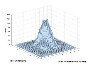
hist3([V1,N],[30,30])
V1 Versus N is the same histogram as randn Versus randn. The only difference is that the axes are labeled. Here are the commands for this
xlabel('Initial Membrane Potential (mV)')
ylabel('Noise Current (nS)')
zlabel('Count')
Now let's try V1 versus V2:
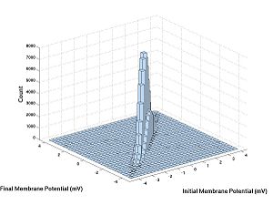
hist3([V1,V2],[30,30])
V1 and N are independent and V1 and V2 are not.
Mathematical Definition of Independence: Two continuous random variables X1 and X2 are independent if and only if their joint density is the product of their marginal densities: p(X1,X2) = p(X1)*p(X2)
- Homework C.1: What is special about the joint density of independent random variables? How can you tell from the second 3D histogram that V1 and V2 are not independent? For this problem, think more about the definition of independence and use it to justify your answer. For more intuition, you could try plotting 3D histograms of other independent random variables [RV1, RV2] where the random variables are functions of different calls to rand or randn (as toward the end of Lab B). This extra work could be the basis of your bonus problem, if you want. See filename conventions.
Joint Densities for Many Random Variables
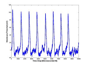
Before we move on let's look a little closer at our Hodgkin-Huxley model and test to see if it is working. You would not ordinarily be interested in just one time step (10 microseconds). Usually you would want the membrane potential on a long sequence of equally spaced times. We can iterate HH1step to draw this picture. Cut and paste the following sets of commands into MATLAB:
N = 0.01;            % Set Noise level
I = 10;              % Set Injected current (mA)
V = zeros(10000,1);  % Allocate memory
V(1) = 0;            % Set Initial membrane potential
The symbol % tells MATLAB to ignore the rest of the line, so you can add a comment to a command. I is the injected current. Without specifying I, as above, the program sets I=0, but this doesn't make a nice voltage trace over 100 milliseconds because the squid axon is quiet without an injected current. Now we make a loop and plot:
[V(2),A] = HH1step(V(1),randn*N,I);
for i = 3:10000
[V(i),A] = HH1step(V(i-1),randn*N,I,A);
end
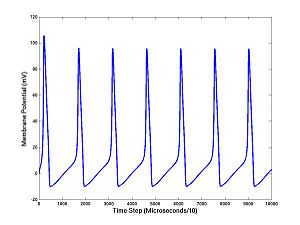
plot(1:10000,V)
You should see a train of action potentials. The first command takes the first step, as before, but returns the ionic current activation variables (A) needed to continue the simulation. If you don't tell HH1step the values of A, it uses defaults; this is done on the first step. But if you continue the simulation you cannot continue to use the defaults: the components of A are changing quantities that, like the membrane potential, are needed for running the model and making predictions. The V's and the A's are the state variables. There are four state variables for the Hodgkin-Huxley equations (V and the three components of A). Notice what we have done with the noise: we add N*randn at each step. (Here is a technical point that is not too important: Inside the program I actually set the standard deviation of the added noise to be the noise level times the square root of the time step: N*randn*sqrt(10 microseconds), which is required for convergence as the time step (10 microseconds in this case) tends to zero.)
This is key: we have added noise at each step of the Hodgkin-Huxley simulation and arrived at a voltage trace. Thus each of the 10000 values of membrane potentials (at successive times separated by 10 microseconds) is a random variable. If the noise level N is large, this is more obivious. You can change I or N easily and rerun:
I = 11;
N = 10;
Now cut and paste the 5 commands above, ending with plot(1:10000,V), into MATLAB, several times, and see how the trajectory differs each time.
Guess what? These random variables (V1,V2,...,V10000) have a joint density: p(V1,V2,...,V10000). You could plot this with a 10000 dimensional histogram! Well, OK, you probably couldn't do that, but theoretically speaking it's conceivable.
Each time you run the program you get V1,V2,...,V10000, a sequence of numbers. These will fall into bins of the 10000 dimensional histogram. The limiting fraction of times that the sequence falls into a small bin, divided by its 10000 dimensional volume, is the joint density, measuring how probable (i.e. probability density) the observed sequence is.
Another key point: If you change I and N, you get a different probability density. In other words, the probability density is a function of I and N. To express this fact it is written p(V1,V2,...,V10000|I,N) but this notation is an abuse of notation because I and N are not random variables.
What if you don't know what I and N are but you ran an experiment and had the numbers V1,V2,...,V10000. That is
I = 10*rand;
N = 10*rand;
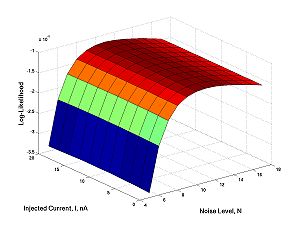
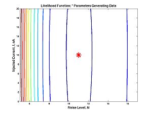
Now repeat the 5 commands that run and plot the model. Now V1,V2,...,V10000 are fixed numbers (what you obtained from the calculation and plotted), but you think of I and N as variables. No more 10000 dimensions: there remain only two! p(N,I). This function is called the likelihood function.
Here is what it looks like (for I=11, N=10):
The peak this function is the maximum likelihood estimate of parameters.
There are somewhat subtle theorems that talk about the convergence of the estimates as the amount of data grows. Maximum likelihood estimation is one of the most well studied methods of parameter estimation in statistics.
Probability Density with randn
Calculating likelihood for the Hodgkin-Huxley model both conceptually difficult and takes a long time (minutes) on a computer. Drawing graphs takes hours. Lets do it for randn (much faster).
Remember the commands for drawing a histogram
A = randn(100000,1);
hist(A,100);
Compare this histogram with the theoretical density for the normal distribution:
x = -5:0.01:5;
density = exp(-x.^2/2)/sqrt(2*pi);
plot(x,density)
Remember what the difference between these two plots is. The histogram measures the count of how many rolls of randn fall into the bin. The pdf normalizes the histogram: it is the fraction of throws that fall into bins, not the count of throws; and it is the limit as the bin size goes to zero divided by the bin size.
It would be nice to have a function that returns the probability density. Type this into the editor and save as randnpdf.m:
function density = randnpdf(x)
% Return density of randn

density = exp(-x.^2/2)/sqrt(2*pi);
Now you can calculate the probability density of any value of randn. Try this
>> randnpdf(0)

ans =

    0.3989

>> randnpdf(1)

ans =

    0.2420

>> randnpdf(2)

ans =

    0.0540
Another thing you can do is get a data point, then see its density
x = randn
randnpdf(x)
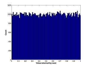
Repeat these commands about 10 times (cut and paste or use the up arrow) to get some intuition about how much probability density points (i.e. calls to randn) tend to have and how much variation there is. Note that if the distribution changes (i.e. use rand instead of randn) this experiment can come out very differently. Specifically all points returned by rand have density 1: remember what the histogram looked like.
Probability Density For Several Calls to randn
You can get an array of the densities for each separately (marginal densities) by typing
>> x = randn(2,1)

x =

    0.6856
   -1.3800

>> densities = randnpdf(x)

densities =

    0.3154
    0.1540
Because two calls to randn are independent, the joint density is the product of the marginal densities
>> jointdensity = prod(densities)

jointdensity =

    0.0486
But there is a problem if we try to do this with 100000 data points: the densities are small numbers, look what happens when we multiply 100000 small numbers together in MATLAB:
>> x = randn(100000,1);
>> densities = randnpdf(x);
>> jointdensity = prod(densities)

jointdensity =

     0
MATLAB cannot represent a number that small, so it gets turned into zero. No matter what the data are, the probability density calculated by MATLAB will be 0.
Solution: We can calculate the log of the joint density. When we calculate likelihood, we will want to compare two different sets of parameter values. Does one set produce more probability density (i.e. likelihood) or does the other? Recall: "A < B" if and only if "log(A) < log(B)", so we might as well just compare log-likelihoods because that is the only thing we can compute in MATLAB. Also recall: log(A*B) = log(A) + log(B). So here is the computation:
>> logjointdensity = sum(log(densities))

logjointdensity =

  -1.4163e+05
You will get a slightly different number depending on the seed of randn.
Repeat the following commands in MATLAB 5 or 6 times and note that there is much less variation in the joint density (or log of joint density) of 100000 calls to randn than there was variation in the density of one call to randn.
x = randn(100000,1);
densities = randnpdf(x);
logjointdensity = sum(log(densities))
This observation is similar to the observation that while the value returned by randn varies, the histogram of 100000 calls to randn varies less.
Likelihood for randn as a function of Mean and Standard Deviation
Remember the probability density function is the probability density as a function of the possible values of a random variable. On the other hand, the likelihood function is the probability density as one or more parameters vary. The noramal distribution has two such parameters mean and standard deviation. To get a random number with mean m and standard deviation s, here is what you do:
First set m and s:
m = 10;
s = 0.1;
Now repeat this command:
s*randn + m
Repeat this command several times. You should get values close to (within several standard deviations from) the mean 10.
Let's create a function. Open the editor and type in the following:
function v = randnms(n,m,s)
% RANDNMS Draw n samples from a normal distribution with mean m, std s

v = s*randn(n,1)+ m;
Save the file as randnms.m and try it out
>> randnms(3,10,.1)

ans =

   10.0896
    9.8811
    9.8484
Now we want the PDF of randnms. This will be another function; in the editor, and cut and paste the following
function density = randnmspdf(x,m,s)
% Return density of randn

density = exp(-(x-m).^2./(2*s.^2))./(s.*sqrt(2*pi));
Now we can draw samples from randnms using a true mean and true standard deviation. If this were data collected in the lab, you might not know what these true parameters are. But you could calculate the likelihood at assumed means and standard deviations. If you did not know the true parameters, your assumed parameters would probably be different:
true_mean = 1.1;
true_std = 2.1;
data = randnms(100000,true_mean,true_std);
assumed_mean = 1;
assumed_std = 2;
densities = randnmspdf(data,assumed_mean,assumed_std);
log_like = sum(log(densities))
Now compare the log-likelihood at the true parameters versus the assumed parameter (and remember that the two were very close). With the data from my random number seed, I get:
>> densities = randnmspdf(data,assumed_mean,assumed_std);
>> log_like = sum(log(densities))

log_like =

  -2.1657e+05

>> densities = randnmspdf(data,true_mean,true_std);
>> log_like = sum(log(densities))

log_like =

  -2.1619e+05
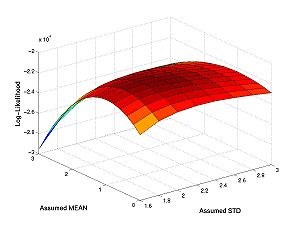
Notice that the true parameters give a greater (slightly less negative) value of likelihood. If we don't know the true values of the parameters, we can estimate them by using the value of the parameters that maximizes likelihood. Let's see what the likelihood function looks like:
The first set of commands set the true parameters, the range of the assumed parameters, and the size of the sample. You can change these numbers and rerun if you want.
true_mean = 1;
true_std = 2;                  % The std must be positive
assumed_means = 0:.2:3;
assumed_stds = 1.6:.2:3;       % The std must be positive
n = 10000;
These statements generate the data and calculate the log-likelihood at each set of parameter values in the range. You can rerun these commands to see if the likelihood function depends on the sample drawn.
data = randnms(n,true_mean,true_std);
loglike = zeros(numel(assumed_means),numel(assumed_stds));
for i = 1:numel(assumed_means)
 for j = 1:numel(assumed_stds)
  densities = randnmspdf(data,assumed_means(i),assumed_stds(j));
  loglike(i,j) = sum(log(densities));
 end
end
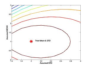
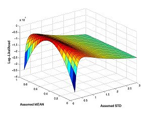
These figures plot the likelihood function as a surface and as a contour. For the figures below I have changed the line widths and marker sizes to project better. These commands are not shown.
figure(1)
surf(assumed_stds,assumed_means,loglike)
figure(2)
contour(assumed_stds,assumed_means,loglike)
hold on
plot(true_std,true_mean,'r*')
hold off
The problem of finding the maximum likelihood estimates of the parameters gets harder and harder the more parameters you do not know. So sometimes when you think you know a parameter pretty well you just assume you know it and it drops out of the likelihood function. The problem is sometimes you get it wrong. This is a big issue for neural models. You are forced to make certain assumptions about the model, but how sensitive are your results on the precise validity of your assumptions? The following three homework problem explores these issues.
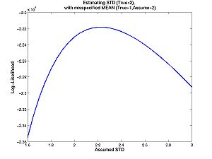
- Homework C.2: Suppose you want to estimate the standard deviation. The true standard deviation is 2 (as above). The true mean is 1 (as above), but you think the mean is 2. Approximately, what is your estimate? It is possible to figure it out from the contour plot above. But it is easier if you plot the one-dimensional likelihood function with the commands below, or just click on the image. Your estimate is the value of standard deviation that maximizes the function. Look carefully at the one dimensional (i.e. one independent variable) plot and the contour plot. How are they related? How is one-dimesional plot embedded in the two dimesional plot? See filename conventions.
true_mean = 1;
true_std = 2;                  % The std must be positive
assumed_mean = 2;
assumed_stds = 1.6:.05:3;       % The std must be positive
n = 10000;

data = randnms(n,true_mean,true_std);
loglike = zeros(1,numel(assumed_stds));
for j = 1:numel(assumed_stds)
 densities = randnmspdf(data,assumed_mean,assumed_stds(j));
 loglike(j) = sum(log(densities));
end

figure(3)
plot(assumed_stds,loglike)
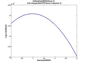
- Homework C.3: Same question, but now you try to estimate the mean, with an incorrect assumption about the standard deviation. The true mean is 1, the true standard deviation is 2, but you assume the standard deviation is 1. What is your estimate? Is maximum likelihood for normal distributions more sensitive to misspecified means or misspecified standard deviations. Why? See filename conventions.
true_mean = 1;
true_std = 2;                  % The std must be positive
assumed_means = 0:.05:3;
assumed_std = 1;              % The std must be positive
n = 10000;

data = randnms(n,true_mean,true_std);
loglike = zeros(numel(assumed_means),1);
for i = 1:numel(assumed_means)
  densities = randnmspdf(data,assumed_means(i),assumed_std);
  loglike(i,1) = sum(log(densities));
end

figure(3)
plot(assumed_means,loglike)
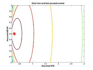
- Homework C.4: What if the data were generated by the "rand" command instead of the "randnms" command we created, based on randn. How well can you estimate the mean and standard deviation? See filename conventions. Clarification added later: This question concerns the plots below. I generated data with the command rand, but calculated the likelihood using a model that incorrectly assumes the data are from randmns.
I replaced the command
data = randnms(n,true_mean,true_std);
With the command
data = rand(n,1);
Then I spent considerable time tweaking the ranges (of the assumed means and stds) to get the plot to look reasonable. Just look at the results below:
- Homework C.*: Bonus Problem (one point). Be creative! See filename conventions.
If you finish lab early, you might want to look at the textbook software, which should be on the lab computers now. Next Thursday's lab will use this software. If it does not work, tell me.
Coming Soon
Here is the present plan:
Thursday, Jan 5: Introduction to Neuron's in a Action, textbook.
Tuesday, Jan 10: Model Selection and Discussion of Projects.
Beyond: More textbook tutorials, and eventually a lab that discussion Bayesian filtering, how likelihood is calculated for the Hodgkin-Huxley model.
