Optimization

First, we discuss homework from Lab V.

Now on to today's topic.

What is Optimization

Given a function that depends upon parameters, find the value of the parameters that optimizes the function (e.g. if the function is likelihood, find the maximum likelihood).

Minimizing functions is trivially the same thing as maximizing functions. Most optimization routines are written to minimize function; if you want to maximize log-likelihood with such a function, you can just minimize minus-log-likelihood. Putting a minus sign in front of the function turns the surface upside down and cost next to nothing computationally.

No Free Lunch!

What is the best optimization routine to use? The "no free lunch" theorem tells you that it doesn't exist; or rather it depends upon your problem. As a result there is a wide diversity of different algorithms that are used in practice. Consider the following rather famous news group post that describes many of the algorithms in a funny way. (OK many of the jokes are inside jokes that only make sense if you already know the algorithms, but the post at least gives you a flavor of the diversity of optimization algorithms.) The post can be found here.

Our Problem

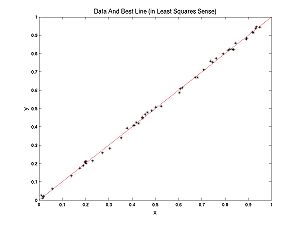
We have some data in the (x,y) plane. Here we consider x to be the independent variable and y to be the dependent variable. Our optimization problem is to find the line y = m*x + b that best fits the data.

Here is some data with the best fitting line.

Click image for full size image

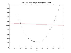
In this case, a line fits well. In the following example a parabola fits better than a line, but we can still ask, what's the best line? The best line is shown:

Click image for full size image

What determines the best line? Each (x,y) pair from the data has an error associated with it for any given parameter pair (m,b): Error(x,y,m,b) = mx + b - y. Each parameter pair (m, b) has a cost associated with it. Customarily this cost is almost always defined as:

$Cost_{LS}(m,b) = \sum_{data} Error(x,y,m,b)^2$

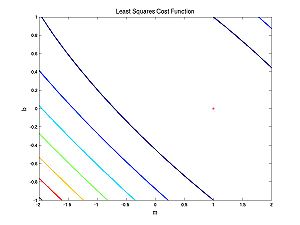
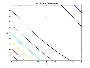
What does this cost function look like as a function of the parameters?

The first case (nearly linear data):

Click image for full size image: cost function for best line fitting nearly linear data

And the second case (nearly parabolic data):

Click image for full size image: cost function for best line fitting nearly parabolic data

Note that both of these cost functions are very well behaved. Fitting a line to data using a least squares (LS) cost function is a very well behaved problem. To give you an idea of what can happen in more general scenarios (i.e. perhaps with maximum likelihood applied to neural models), I have cooked up a different cost function:

$Cost_{UG}(m.b) = \sum_{data} (1 - exp(-\frac{Error(x,y,m,b)^2}{dev^2}))$

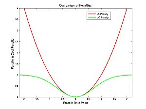
The difference between the cost functions is how they penalize errors. The LS cost function uses squared error whereas the UG one uses an upside-down Gaussian:

Click image for full size.

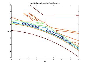
You might naively choose to use the UG cost function to avoid overly penalizing outliers. The problem with this is apparent from the following image of the UG cost function for the nearly parabolic data:

Click image for full size image: UG cost function for best line fitting nearly parabolic data

There is no longer just one peak or trough but lots of little ones. This makes optimization very hard. But we will talk about the way around it. The little peaks or troughs are called local maxima or minima. Next we will talk about an optimization method that is appropriate if you are not worried about local maxima.

The Nelder-Meade Method

The Nelder-Meade method is appropriate if you are not worried about getting caught in local (non-global) extrema. Nelder-Meade assumes that the only tool you have is the evaluation of the function at any values of the parameters. For example, it does not assume that you can evaluate the derivatives. Much faster methods exist if you can.

• Because we have two parameters (m and b), we start with 3 points, chosen arbitarily (3 kangaroos). If we had n parameters, we would use n+1 points (n+ 1 kangaroos).

• Take the worst point (e.g. the kangaroo with the lowest likelihood), and reflect it across the line (plane, hyperplane, etc) determine by the other points.

• If the reflected point is no longer the worst, but neither the best, repeat the above step with the new worst point.

• If on the other hand the reflected point is now the best, take a larger step.

• If on the other hand the reflected point is still the worst, take a smaller step, and if that doesn't work, shrink the triangle (move all kangaroos) on the assumption that it spans the desired optimum.

And there you have it (basically, sometimes details differ).

When you care about local optima: Nelder-Meade Modified for Simulated Annealing

The trick here is to add noise to your evaluations of the function. What this means is you go in the wrong direction sometimes. The amount of noise you add, depends on a quantity called "temperature" which slowly decreases to zero. When it gets to zero there is no longer any noise added. An analogous situation happens when atoms find their perfect crystaline structure (lowest energy configuration) as the temperature (and thermal noise) decreases. If the cooling of an annealing crystal happens to rapidly (quenching) a nonoptimal crystaline structure is found.

The critical quantity is the cooling schedule. Cool too quickly and you get bad results, too slowly and it takes forever.