Difference between revisions of "Bayesian Filtering"
| Line 3: | Line 3: | ||
<math> O \rightleftharpoons C \rightleftharpoons S </math> | <math> O \rightleftharpoons C \rightleftharpoons S </math> | ||
| − | Transitions between O and S never happen (i.e. the probability is negligible) without C being an intermediary state. The observed current is zero in C and S and one in O. And there is noise. We want to estimate the | + | Transitions between O and S never happen (i.e. the probability is negligible) without C being an intermediary state. The observed current is zero in C and S and one in O. And there is noise. We want to estimate the transition probabilities. (The probabilities will depend upon the time step, but say the time step is fixed). |
First generate some data which looks like. | First generate some data which looks like. | ||
| Line 22: | Line 22: | ||
Probability(Stuck -- Closed) = 0.003 | Probability(Stuck -- Closed) = 0.003 | ||
Probability(Stay in Stuck) = 0.097 | Probability(Stay in Stuck) = 0.097 | ||
| + | |||
| + | There are nine parameters here, but there is a constraint that each block add to 1, so we only have 6 parameter to estimate. Moreover we might know that transition between open and stuck never happen, so there would only be 4 parameters to estimate. | ||
| + | |||
| + | Thus the likelihood function is a function from four parameters to one value (likelihood). Too many to plot. Let's say we know the probabilities of going back and forth between open and closed. Thus we need only know the probabilities of going back and forth between closed and stuck. These are the invisible transitions because they cause no change of conductance. | ||
Revision as of 00:24, 8 April 2009
Here is the problem -- there is an open state (O) and closed state (C) and a stuck (inactivated) state (S). Transitions between these states happen like this

Transitions between O and S never happen (i.e. the probability is negligible) without C being an intermediary state. The observed current is zero in C and S and one in O. And there is noise. We want to estimate the transition probabilities. (The probabilities will depend upon the time step, but say the time step is fixed).
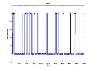
First generate some data which looks like.
The transition probabilities for this plot are
Probability(Stay in Open) = 0.95
Probability(Open --> Closed) = 0.05
Probability(Open --> Stuck/Inactive) = 0.00

Probability(Closed --> Open) = 0.10
Probability(Stay in Closed) = 0.85
Probability(Closed --> Stuck) = 0.05

Probability(Stuck --> Open) = 0.00
Probability(Stuck -- Closed) = 0.003
Probability(Stay in Stuck) = 0.097
There are nine parameters here, but there is a constraint that each block add to 1, so we only have 6 parameter to estimate. Moreover we might know that transition between open and stuck never happen, so there would only be 4 parameters to estimate.
Thus the likelihood function is a function from four parameters to one value (likelihood). Too many to plot. Let's say we know the probabilities of going back and forth between open and closed. Thus we need only know the probabilities of going back and forth between closed and stuck. These are the invisible transitions because they cause no change of conductance.
