Selection

First, the homework from Lab W.

What is Model Selection?

What is model selection? To answer this question let's contrast model selection with parameter estimation. In the Optimization Lab, we fit lines to data. We were doing parameter estimation, trying to estimate the parameters m and b, in the formula for a line y = m*x + b. Recall my examples: we fit a line to nearly linear data and another line to nearly parabolic data.

Fitting a line to nearly linear data. Click for full size image

Fitting a line to nearly parabolic data. Click for full size image

Clearly, in the second case, it would be more appropriate to fit a parabola to the data, rather than a line. How would we do that?

A parabola is described by the formula: 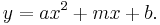$y = a x^2 + m x + b.$ This is a line with a new term, $a x^2,$ added. To fit a parabola the procedure is almost the same. First determine the errors in the data:

$Error(x,y,a,m,b) = a x^2 + m x + b - y$

Now define the penalties, (let's be sensible and use LS rather the UG penalties):

$Penalty(x,y,a,m,b) = Error(x,y,a,m,b)^2$

And finally the cost function

$Cost(a,m,b) = \sum_{data} Penalty(x,y,a,m,b)$

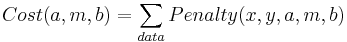
Now we tweak the three parameters (a,m,b) using, for example, the Nelder-Meade method we studied last week. Of course MATLAB has its own routines for solving this problem based on Linear Algebra that are much better than Nelder-Meade.

What if we fit a parabola to the nearly linear data? Note that if we set a = 0, we get y = m*x + b again. Thus a line is a parabola. But there was some noise in the data, so if you are allowed to tweak the parameter a as well as m and b, you can expect a better (lower cost) fit (you are guaranteed that the fit is no worse). So why should we bother fitting lines to data? Why not just always fit parabolas?

But wait, why stop at parabolas? An nth degree polynomial has the form:

$y = a_n x^n + a_{n-1} x^{n-1} + \dots + a_1 x + a_0$

For example, a 0th degree polynomial is a constant function, 1st degree is a line, 2nd degree is parabola, etc. If we have m data points a unique polynomial of degree m-1 will fit exactly (provided the x-values of the data points are not repeated). Some (no longer unique) higher degree polynomials will also fit exactly under the same stipulation.

So why don't we fit with a high enough polynomial so that there is no error? If we have 100 data points why not use a 99 degree polynomial? Then there is no errors, no penalties, and zero cost! Perfect fit!?

There are two reasons you don't want to do that:

• Philosophical: parsimony. The model that generated our data (in both examples above) is a low degree polynomial plus noise. This model can be described with only a few parameters (a,m,b) and NoiseLevel. If our data is generated in the lab, we may never know what the exact model is that created the data. But Occam's razor (a standard paradigm in science) tells us we should pick the simplest model that is consistent with the data. The complexity of a model can be quantified with number of parameters. A degree m polynomial has m+1 parameters. Thus a low degree polynomial is preferred unless the data compel the use of a more complicated model.

• Practical: overfitting (subject of next section). Fitting models with too many parameters leads to fits that are tuned in a sensitive way (overfitted) to the particular noise that appeared in the data set used for the fitting. If you run the experiment again, you get different noise. Typically, an overfitted model does a much worse job of predicting the new experiment (with new noise) than a simpler more parsimonious model.

Model selection helps you decide how complicated a model you need to fit the data in a way that is robust to repeating the experiment. What we are going to do today is generate some data (polynomial plus noise) then use Model Selection to decide what degree fits the data best.

For neural models, you might use model selection to decide how many currents, and what types of currents are present in a cell, or how many compartments are needed in a multi-compartment model to reproduce the data.

Model Selection Statistics

We will use two satistics:

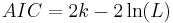
• The Akaike Information Criterion (AIC).

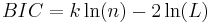
• The Bayesian Information Criterion (BIC).

There are more.

The formula for these statistics are

$AIC = 2 k - 2 \ln(L)$

$BIC = k \ln(n) - 2 \ln (L)$

where

• k is the number of parameters (degree of polynomial plus 1)

• L is the maximum value of the likelihood (related to the minimizing LS-Cost by a simple formula: likelihood = "a negative constant"*LS-cost)

• n is the number of data points (used for BIC but not for AIC)

The model with the lowest AIC or BIC wins. Note that the statistics is a simple tradeoff between fewer parameters and greater likelihood.

If you are comparing an infinite family of models, such as polynomials of all degrees, you need a model selection strategy. This is the one I used:

• Start with degree 0 (constant function). Calcuate selection statistic.

• Increase degree, recalculate statistic. If statistic is lower (better model) keep going.

• Repeat previous step until you get a higher statistic (worse model), at which point you stop and the best model so far (second to last) wins.

Following this steps you don't need to try infinitely many degrees.

Homework

Homework X.1 For our class of problems when does model selection work well, and when does it work poorly? Try different combinations of low/high levels of noise, and lots of/few data points. For this part, use a fairly simple polynomial to generate the data. Note: I don't know what will happen if you try to fit polynomial with degree higher than the number of data points. Maybe an error.

Homework X.2 Investigate the effects of the polynomial's shape on model selection. Get creative!