Optimization
First, we discuss homework from Lab V.
Now on to today's topic.
Contents
[hide]What is Optimization?
Given a function that depends upon parameters, the optimization problem is to find the value of the parameters that optimizes (meaning, in different contexts, either minimizes or maximizes) the function. For example, if the function is likelihood, you want to find the maximum likelihood.
Minimizing functions is trivially the same thing as maximizing functions. Most optimization routines are written to minimize functions; if you want to maximize log-likelihood with such a routine, you can just minimize minus-log-likelihood. Putting a minus sign in front of the function turns the surface upside down and costs next to nothing computationally.
No Free Lunch!
What is the best optimization routine to use? The "no free lunch" theorem tells you that it doesn't exist; or rather it depends upon your problem. As a result there is a wide diversity of different algorithms that are used in practice. Consider the following rather famous news group post that describes many of the algorithms in a funny way. (OK many of the jokes are inside jokes that only make sense if you already know the algorithms, but the post at least gives you a flavor of the diversity of optimization algorithms.) The post can be found here.
Our Problem
We have some data in the (x,y) plane. Here we consider x to be the independent variable and y to be the dependent variable. Our optimization problem is to find the line y = m*x + b that best fits the data.
Here is some data with the best fitting line.

In this case, a line fits well. In the following example a parabola fits better than a line, but we can still ask, what's the best line? The best line is shown:

What determines the best line? Each (x,y) pair from the data has an error associated with it for any given parameter pair (m,b): Error(x,y,m,b) = mx + b - y. Each error has a penalty associated with it; customarily this is the square of the error. Each parameter pair (m, b) has a cost associated with it, customarily the sum of the penalties:

What does this cost function look like as a function of the parameters?
The first case (nearly linear data):

And the second case (nearly parabolic data):

Note that both of these cost functions look similar. Fitting a line to data using a least squares (LS) cost function is a very well behaved problem no matter what the data. To give you an idea of what can happen in more general scenarios (i.e. perhaps with maximum likelihood applied to neural models), I have cooked up a different cost function:
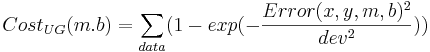
The difference between the cost functions is how they penalize errors. The LS cost function uses a squared-error penalty whereas the UG cost function uses an upside-down Gaussian:

You might naively choose to use the UG cost function to avoid overly penalizing outliers. The problem with this is apparent from the following image of the UG cost function for the nearly parabolic data:

There is no longer just one peak or trough but lots of little ones. This makes optimization very hard. But we will talk about the way around it. The little peaks or troughs are called local maxima or minima. Next we will talk about an optimization method that is appropriate if you are not worried about local maxima.
The Nelder-Meade Method
The Nelder-Meade method is appropriate if you are not worried about getting caught in local (non-global) extrema. Nelder-Meade assumes that the only tool you have is the evaluation of the function at any values of the parameters (i.e. the kangaroos only have altimeters). For example, it does not assume that you can evaluate the derivatives. Much faster methods exist if you can.
- Because we have two parameters (m and b), we start with 3 points, chosen arbitarily (3 kangaroos). If we had n parameters, we would use n+1 points (n+ 1 kangaroos).
- Take the worst point (e.g. the kangaroo with the lowest likelihood), and "reflect" it across the line (plane, hyperplane, etc) determine by the other points.
- If the reflected point is no longer the worst, but neither the best, repeat the above step (reflect) with the new worst point.
- If on the other hand the reflected point is now the best, take a larger step ("expand").
- If on the other hand the reflected point is still the worst, take a smaller step ("contract"), and if that doesn't work, "shrink" the triangle (move all kangaroos) on the assumption that the optimum lies inside the triangle.
And there you have it (basically, sometimes details differ).
When you care about local optima: Nelder-Meade Modified for Simulated Annealing
The trick here is to add noise to your evaluations of the function (i.e noisy altimeter). What this means is you go in the wrong direction sometimes (drunk kangaroo). The noise can get you out of a bad optimum and into a better one (that's more likely than going from a good to a bad). The amount of noise you add depends on a quantity called "temperature" which slowly decreases to zero (kangaroo sobers up). When it gets to zero there is no longer any noise added. An analogous situation happens when atoms find their perfect crystaline structure (lowest energy configuration) as the temperature (and thermal noise) decreases. If the cooling of an annealing crystal happens too rapidly (quenching) a nonoptimal semi-crystaline structure is found.
The critical quantity is the cooling schedule. Cool too quickly and you get bad results, too slowly and it takes too long.
Animating the Nelder-Meade Method
First, download the zip file. Or download the files individually:
The next thing to do is to generate some data. At the MATLAB prompt (with the above files in your PATH), type
pdata = GenPolyData;
The variable pdata will store the data you generate. Now the function will open a figure and hang. Move the mouse into the figure and click somewhere inside the axes (x & y both between 0 & 1). This will draw a point and a constant function through that point. The next time you click it will draw a line through the two points, and then a parabola through the three, and so on. When you are done, click inside the figure but outside the axes. That sets the function that generates the data. Now enter a noise level, number of points and random seed and it plots data and returns your variable with the data. Type
pdata
to see the variable. It is a stucture. To see the fields of the stucture (for example, Seed) type
pdata.Seed
Thus using the '.' you can access the fields of a structure. But you won't need to .. just pass the structure (pdata) onto the other programs.
The next thing to do is determine the best line in the LS-sense:
BestLineLS(pdata)
This draws the best-LS line and also returns the best-LS (m,b) in the text window.
Now decide on a range for m and for b for plotting the cost function:
mrange = -3:.1:3;
brange = -3:.1:3;
Plot the LS-Cost Function
LSplot(mrange,brange,pdata);
You can plot the true optimum using the commands
m = ??????; % CUT AND PASTE m FROM THE OUTPUT OF BestLineLS
b = ??????; % CUT AND PASTE b FROM THE OUTPUT OF BestLineLS
hold on
plot(m,b,'g*');
Now set up the Annealing. Set up an initial condition (a starting point for the optimization). This can be anything. I chose
m0 = -2;
b0 = -2;
Now set up the options to Anneal:
options = AnnealSet('Display','anim','Schedule','quench');
This says we want an animation of the results and for the cooling schedule, just quench. Now run the optimization:
bestmb = Anneal('LScost',[m0,b0],options,pdata);
At each step you must press ENTER to continue.
After finishing the optimization, compare the bestmb with the mb returned by BestLineLS. BestLineLS uses linear matrix algebra to solve for the least squares optimum -- BestLineLS uses what is probably the best algorithm for the problem. Anneal also works but is slower.
If you don't want to animate, set options as follows, then run:
options = AnnealSet('Display','iter','Schedule','quench');
bestmb = Anneal('LScost',[m0,b0],options,pdata);
Now we can try the UG-Cost function. It depends on a parameter dev. The larger dev the bigger the region where UG behaves similar to LS thus the less problematical our new cost function is. The smaller dev, the more problematical. I used dev's around 0.2. First we probably will need a finer mesh to resolve the sharp corners in the UG-Cost function. We'll try 0.01, but this might not be fine enough;
mrange = -3:0.01:3;
brange = -3:0.01:3;
dev = 0.2;
Now plot
UGplot(mrange,brange,pdata,dev);
Who knows where the global optimum of this function is. Lets try an annealing with quench. The differences in the Anneal command below are that (1) 'UGcost' is used instead of 'LScost' and dev is passed as a parameter.
options = AnnealSet('Display','anim','Schedule','quench');
bestmb = Anneal('UGcost',[m0,b0],options,pdata,dev);
The UG-Cost function has regions where it is constant to numerical error. If you start it there it won't move. I had to adjust the initial condition:
m0 = -2;
b0 = 1;
bestmb = Anneal('UGcost',[m0,b0],options,pdata,dev);
Now lets try running with annealing turned on (that is, quench turned off)
options = AnnealSet('Display','anim');
bestmb = Anneal('UGcost',[m0,b0],options,pdata,dev);
Finally, let's talk about adjusting the cooling schedule. The possible parameters to tweak (through AnnealSet.m) are:
- 'tinitial': starting temperature (must be nonnegative) (default = 1)
- 'tfactor': factor to reduce temperature at each cooling step (default = .9). Make this parameter between 0 and 1 (noninclusive)
- 'numsteps': number of cooling steps to take, (default 60)
- 'restart': restart the optimization at the best point (new triangle) every this many cooling steps (default 15). This prevents the annealing from getting hopelessly lost in a bad region of parameter space.
The following parameters tell you when a cooling step is over
- 'maxiter': maximum number of iterations (changes in triangle) per cooling step (default ='15*numberOfVariables' or 30 in our case)
- 'maxfunevals': maximum number of function evaluations per cooling step (default = '15*numberOfVariables', or 30 in our case)
- 'qfactor': last step is a quench, increase maxiter and maxfunevals by this factor for last step (default 15)
If you want to change all the parameters, use the following command (broken up into several lines)
options = AnnealSet('Display','iter','tinitial',2,...
'tfactor',0.5,'numstep',10,'restart',5,...
'maxiter',40,'maxfunevals',40,'qfactor',20);
bestmb = Anneal('UGcost',[m0,b0],options,pdata,dev);
To leave any of these parameters at their default values, just leave them out of the list.
Homework
Homework W.1: First go through today's tutorial. Generate some data and plot the LScost function. Try to find an LScost function with more than one optimum. (I think this is impossible so it's OK if you can't find one). Plot (1) the data and best fitting line and (2) the cost function. Put both plots into your PowerPoint.
Homework W.2: Run Anneal in quench mode, with Animate. How many function evaluations were needed? Print the final image and put into PowerPoint,
Homework W.3: Use UG cost function to come up with a hard problem for optimization. Run Anneal with quench and 3 cooling schedules (fast, medium, and slow) and compare results. The results will depend on your problem.