NumHH
It has come to my attention that there is a related class (in Mathematics) being taught at Hopkins.
Lets look at the Lab H Homework.
Moving on to today's material, recall that we have looked at the action potential with the Hodgkin-Huxley model using the textbook software, Neurons in Action. Today we are going to use MATLAB. We will generate data, then change parameters, then calculate the likelihood that the model (with different parameters) produced the data.
Contents
Time Step Function
Here is the function that simulates the model (one step at a time):
function nextState = hh_step_template(state,input,noise,param)

alpha_m = (2.5 - 0.1*stateV)./(exp(2.5 - 0.1*stateV) - 1);
alpha_n = (0.1 - 0.01*stateV)./(exp(1 - 0.1*stateV) - 1);
alpha_h = 0.07*exp(-stateV./20);
beta_m = 4*exp(-stateV./18);
beta_n = 0.125*exp(-stateV./80);
beta_h = 1./(exp(3-0.1*stateV)+1);

ionicCurrent = gNa*stateM^3*stateH*(stateV-ENa) ...
     + gK*stateN^4*(stateV-EK) ...
     + gL*(stateV-EL);

nextState = [stateV + oneDT./CAP*(injectedCurrent - ionicCurrent) ...
                    + sqrtDT*PNoiseLevel*PNoise; ...
             stateM + oneDT*(alpha_m*(1-stateM) - beta_m*stateM); ...
             stateN + oneDT*(alpha_n*(1-stateN) - beta_n*stateN); ...
             stateH + oneDT*(alpha_h*(1-stateH) - beta_h*stateH)];
This function returns the nextState (state at current time plus oneDT) as a function of current state (stateV,stateM,stateN,stateH) input (injectedCurrent) noise (PNoise) and parameters (param).
Note that this function won't run because a lot of things (like injectedCurrent and ENa) aren't defined. A function like this one can be very hard to make both human readable and run quickly. So I have written preprocessor CreateCell.m which takes the human readable template function above and creates machine readable MATLAB Code function, based on a key function, HH.m.
Before we discuss the key function the nextState equation requires explanation:
nextState = previousState + oneDT * f(previousState)
This is a famous equation known as Euler's method to approximate solutions to the differential equation:
d(state)/dt = f(state)
Lets look at Euler's method next.
Numerical Solution of Differential Equations
Remember the equation for the cell with only leak channels.
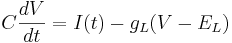
Let's simplify: suppose there is no injected current and that the reversal potential for the leak channels is  . Then our equation is
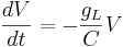
Using different letters for the variables (because this is done in the software linked below):

Here k is the rate constant, 1/k is the time constant, 1/k is  in the notation above. A leaky cell is what is called an RC circuit -- a resistor and capacitor together in a circuit. The time constant of an RC circuit is RC. The bigger k, the higher the rate of convergence, and the smaller the time constant 1/k. The time constant is the time it takes the solution to decay to 1/e of its value.
Solution of differential equations happens at discrete times:  , separated by small time intervals
  .
.
The simplest way of solving this equation is with Euler's method:
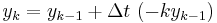
This is a special case of the general formula for Euler's method applied to the (vector) differential equation

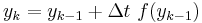
Euler's equation is the simplest way to solve a differential equation numerically. However it is often not the preferred method: often you need to take much smaller time steps with Euler than with some other methods, so it takes longer to get as good a solution. Still if you are doing something complicated, like solving an equation with noise, or Bayesian filtering (to compute likelihood), an argument can be made that a simpler method is desirable -- at least as a first step.
Click here for NEURON code for visualizing the numerical solution of differential equations. Find the file icon in the SaveFilesHere directory and double click on it.
Creating Models From The Key and Template Files
Download the following (or the zip file, see note below):
- HH_step_template.m: This is the function that steps from one time to the next.
- HH_meas_template.m: This is the function that models the measurement of the membrane potential with noise.
- HH.m This is the key file.
- CreateCell.m: This it the function that converts the key and template files into the MATLAB code files.
Now type
CreateCell(HH)
This creates five files (you don't need to download these):
If you change the template or the key you get a different set of 5 functions. That's the whole point. The "gen" functions are for generating data. The "fit" functions are for fitting the model to data. The point is the model used to generate data can be different from the one used for fitting. The "ics" function returns the initial conditions (parameters, state for generating, and state for fitting). The next step is to create the data. For this you need two more functions
- StepCurrent.m: This function creates a step current input.
- CreateData.m: This function creates the data.
To create the data, execute the following command:
CreateData(HH)
This creates and plots data (input and measurements as a function of time). It saves the data in the file HH.mat, (the filename is the "prefix" in the key file). If you load the saved file, you can plot other things (like the state variable, stateM, with the commands:
load HH
plot(out.time,out.stateM)
After loading HH, type
out
For a list of things you can plot).
The final step of the process is the likelihood calculation. For this you need two functions, plus Freeware code that it uses.
- EKFit.m: The function that does the filtering. (We will talk about what this function does in a future lecture.)
- CalcLike.m: This function provides a more user friendly way of accessing the filtering function.
Then type
addpath [THEN THE DIRECTORY PATH TO FREEWARE CODE myAD/]
CalcLike(HH)
And you get the likelihood of the assumed parameters specified in the key file. We'll change those in a minute.
Note: Instead of downloading all files separately, you can just download a zip file with the class code and the Freeware code.
Changing the Key File
Let's look at the key file:
function key = HH
% PREFIX TO START FILE NAMES
key.prefix = 'HH';
The first item is the prefix of the files associated with the key (not including the templates). When you change the key, change the name and the prefix. For example change HH.m to HHA.m and prefix to 'HHA'.
% TEMPLATES TO CONVERT TO FAST RUNNING CODE
key.steptemplate = 'HH_step_template.m';
key.meastemplate = 'HH_meas_template.m';
These are the templates. A future version will have separate templates for generation and fitting.
% PARAMETERS FOR GENERATING DATA
key.gen.gNa = 120;
key.gen.gK  = 36;
key.gen.gL  = 0.3;
key.gen.ENa = 115;   % mV
key.gen.EK  = -12;   % mV
key.gen.EL  = 10.6;  % mV
key.gen.CAP = 1;     % uF/cm^2
key.gen.PNoiseLevel = 0.01;
key.gen.MNoiseLevel = 0.001;
These are the parameters for generating the data (not necessarily fitting).
% INITIAL CONDITIONS FOR STATE VARIABLES
key.state.stateV = 0;
key.state.stateM = 0.05293421762087;
key.state.stateN = 0.31768116757978;
key.state.stateH = 0.59611104634676;
These are the state variables and their initial conditions.
% WHICH PARAMETERS TO FIT
key.fit = {'gNa','gK'};
These are the parameters to tweak for finding the maximum likelihood.
% ASSUMPTIONS ABOUT PARAMETERS & STATES, IF NOT SPECIFIED ASSUMED CORRECT
key.assume.gNa = 125;
key.assume.gL = 0.5;
key.assume.stateV = 1;
These are the (possibly) incorrect assumptions about the parameters and initial conditions for fitting.
% INPUT VARIABES AND CODE FOR CREATING INPUT
key.input = {'injectedCurrent'};
key.inputcreate = {@StepCurrent};
key.inputparams(1).holding = 0;
key.inputparams(1).step = 10;
key.inputparams(1).start = 10;
key.inputparams(1).stop = 25;
This specifies the injected current input.
% NOISE VARIABLES
key.noise.process = {'PNoise'};
key.noise.measurement = {'MNoise'};
This specifies the number and names of the noise variables.
% MEASUREMENTS
key.meas = {'measuredVoltage'};
This specifies the number and names of of the measured variables
% TRAJECTORY TIME PARAMETERS
key.time.oneDT = 0.01;    % msec
key.time.sqrtDT = 0.1;    % msec^(1/2)
key.time.TMAX = 30;       % msec
key.time.fitStart = 9;    % msec
These specify trajectory parrameters. sqrtDT must be the square root of oneDT.
% RANDOM SEED
key.seed = 0;
This specifies the seed of the random number generator when generating data.
% DEBUGGING
key.debug = {'ionicCurrent','alpha_m','alpha_n','alpha_h', ...
                            'beta_m','beta_n','beta_h'};
These are the intermediate variables to save while generating data.
Homework
The first 4 questions are worth 1 point each. You are encouraged to check with your classmates and with me to see that we are all getting the same results.
- Homework I.1: Calculate the log likelihood with the default values in the key (follow directions above).
- Homework I.2: Repeat the log-likelihood calculation but change the key so that the fitting makes all correct assumptions (change the values of key.assume to match their values higher up. If there is no assumption about a variable it is assumed correct. You can add or remove assumptions, but you need at least one.
- Homework I.3: Calculate the log-likelihood that an RC circuit (i.e. a cell with just a leak current), produces the action potential data from the Hodgkin-Huxley model. To do this set key.assume.gNa = 0 and key.assume.gK = 0, and remove all other assumptions, and run the code. Please try to understand what you are doing.
- Homework I.4: Calculate the log-likelihood that the voltage trace from a Hodgkin-Huxley model looks identical to one from an RC-circuit. Make key.assume for gNa and gK be the default Hodgkin-Huxley parameters, but for generating the data key.gen.gNa, key.gen.gK, set these to zero.
The last question is worth 6 points and full credit is not automatic. Review question.
- Homework I.5 Concisely and effectively explain the mechanisms behind the action potential.