Difference between revisions of "NumHH"
| Line 1: | Line 1: | ||
| + | We have looked at the action potential with the Hodgkin-Huxley model using the textbook software, Neurons in Action. Today we are going to use MATLAB. We will generate data, then change parameters, then calculate the likelihood that the model (with different parameters) produced the data. | ||
| + | |||
| + | Here is the function that simulates the model (one step at a time): | ||
| + | |||
| + | |||
| + | |||
== Numerical Solution of Differential Equations == | == Numerical Solution of Differential Equations == | ||
Revision as of 19:51, 23 February 2009
We have looked at the action potential with the Hodgkin-Huxley model using the textbook software, Neurons in Action. Today we are going to use MATLAB. We will generate data, then change parameters, then calculate the likelihood that the model (with different parameters) produced the data.
Here is the function that simulates the model (one step at a time):
Numerical Solution of Differential Equations
Remember the equation for the cell with only leak channels.
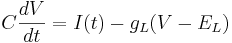
Let's simplify: suppose there is no injected current and that the reversal potential for the leak channels is  . Then our equation is
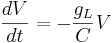
Using different letters for the variables (because this is done in the software linked below):

Here k is the rate constant, 1/k is the time constant, 1/k is  in the notation above. A leaky cell is what is called an RC circuit -- a resistor and capacitor together in a circuit. The time constant of an RC circuit is RC. The bigger k, the higher the rate of convergence, and the smaller the time constant 1/k. The time constant is the time it takes the solution to decay to 1/e of its value.
Solution of differential equations happens at discrete times:  , separated by small time intervals dt.
The simplest way of solving this equation is with Euler's method:
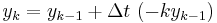
This is a special case of the general formula for Euler's method applied to the (vector) differential equation

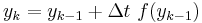
Euler's equation is the simplest way to solve a differential equation numerically. However it is often not the preferred method: often you need to take much smaller time steps with Euler than with some other methods, so it takes longer to get as good a solution. Still if you are doing something complicated, like solving an equation with noise, or Bayesian filtering (to compute likelihood), an argument can be made that a simpler method is desirable -- at least as a first step.
Click here for code for visualizing the numerical solution of differential equations.