Difference between revisions of "Matlab Primer"
| Line 2: | Line 2: | ||
My name is Sean Carver; I am a research scientist in Mechanical Engineering. I have been programming in MATLAB for almost 20 years and programming computers for almost 30 years. | My name is Sean Carver; I am a research scientist in Mechanical Engineering. I have been programming in MATLAB for almost 20 years and programming computers for almost 30 years. | ||
| + | |||
| + | ====Pendulum on a movable support==== | ||
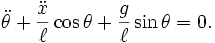
| + | Consider a pendulum of mass ''m'' and length ''ℓ'', which is attached to a support with mass ''M'' which can move along a line in the ''x''-direction. Let ''x'' be the coordinate along the line of the support, and let us denote the position of the pendulum by the angle ''θ'' from the vertical. | ||
| + | |||
| + | [[File:pendulumWithMovableSupport.svg|thumb|right|300px|Sketch of the situation with definition of the coordinates (click to enlarge)]] | ||
| + | |||
| + | The kinetic energy can then be shown to be | ||
| + | |||
| + | :<math> | ||
| + | \begin{align} | ||
| + | T &= \frac{1}{2} M \dot{x}^2 + \frac{1}{2} m \left( \dot{x}_\mathrm{pend}^2 + \dot{y}_\mathrm{pend}^2 \right) \\ | ||
| + | &= \frac{1}{2} M \dot{x}^2 + \frac{1}{2} m \left[ \left( \dot x + \ell \dot\theta \cos \theta \right)^2 + \left( \ell \dot\theta \sin \theta \right)^2 \right], | ||
| + | \end{align}</math> | ||
| + | |||
| + | and the potential energy of the system is | ||
| + | |||
| + | :<math> V = m g y_\mathrm{pend} = - m g \ell \cos \theta . </math> | ||
| + | |||
| + | The Lagrangian is therefore | ||
| + | |||
| + | <math> | ||
| + | \begin{align} | ||
| + | L &= T - V \\ | ||
| + | &= \frac{1}{2} M \dot{x}^2 + \frac{1}{2} m \left[ \left( \dot x + \ell \dot\theta \cos \theta \right)^2 + \left( \ell \dot\theta \sin \theta \right)^2 \right] + m g \ell \cos \theta \\ | ||
| + | &= \frac{1}{2} \left( M + m \right) \dot x^2 + m \dot x \ell \dot \theta \cos \theta + \frac{1}{2} m \ell^2 \dot \theta ^2 + m g \ell \cos \theta | ||
| + | \end{align} | ||
| + | </math> | ||
| + | |||
| + | Now carrying out the differentiations gives for the support coordinate ''x'' | ||
| + | |||
| + | :<math>\frac{\mathrm{d}}{\mathrm{d}t} \left[ (M + m) \dot x + m \ell \dot\theta \cos\theta \right] = 0, </math> | ||
| + | |||
| + | therefore: | ||
| + | |||
| + | :<math> (M + m) \ddot x + m \ell \ddot\theta\cos\theta-m \ell \dot\theta ^2 \sin\theta = 0 </math> | ||
| + | |||
| + | indicating the presence of a constant of motion. Performing the same procedure for the variable <math>\theta</math> yields: | ||
| + | |||
| + | :<math>\frac{\mathrm{d}}{\mathrm{d}t}\left[ m( \dot x \ell \cos\theta + \ell^2 \dot\theta ) \right] + m \ell (\dot x \dot \theta + g) \sin\theta = 0;</math> | ||
| + | |||
| + | therefore | ||
| + | |||
| + | :<math>\ddot\theta + \frac{\ddot x}{\ell} \cos\theta + \frac{g}{\ell} \sin\theta = 0.\, </math> | ||
| + | |||
| + | These equations may look quite complicated, but finding them with Newton's laws would have required carefully identifying all forces, which would have been much harder and more prone to errors. By considering limit cases, the correctness of this system can be verified: For example, <math>\ddot x \to 0</math> should give the equations of motion for a pendulum which is at rest in some [[inertial frame]], while <math>\ddot\theta \to 0</math> should give the equations for a pendulum in a constantly accelerating system, etc. Furthermore, it is trivial to obtain the results numerically, given suitable starting conditions and a chosen time step, by [[Numerical ordinary differential equations|stepping through the results iteratively]]. | ||
Revision as of 21:09, 2 November 2012
Today's lecture will be on MATLAB and PENDULA (plural of PENDULUM). Your next lab assignment motivated the topic.
My name is Sean Carver; I am a research scientist in Mechanical Engineering. I have been programming in MATLAB for almost 20 years and programming computers for almost 30 years.
Pendulum on a movable support
Consider a pendulum of mass m and length ℓ, which is attached to a support with mass M which can move along a line in the x-direction. Let x be the coordinate along the line of the support, and let us denote the position of the pendulum by the angle θ from the vertical.
The kinetic energy can then be shown to be
![\begin{align}
T &= \frac{1}{2} M \dot{x}^2 + \frac{1}{2} m \left( \dot{x}_\mathrm{pend}^2 + \dot{y}_\mathrm{pend}^2 \right) \\
&= \frac{1}{2} M \dot{x}^2 + \frac{1}{2} m \left[ \left( \dot x + \ell \dot\theta \cos \theta \right)^2 + \left( \ell \dot\theta \sin \theta \right)^2 \right],
\end{align}](/images/math/6/1/5/6154d0ab1b938bd2b7753379ed10dda3.png)
and the potential energy of the system is

The Lagrangian is therefore
![\begin{align}
L &= T - V \\
&= \frac{1}{2} M \dot{x}^2 + \frac{1}{2} m \left[ \left( \dot x + \ell \dot\theta \cos \theta \right)^2 + \left( \ell \dot\theta \sin \theta \right)^2 \right] + m g \ell \cos \theta \\
&= \frac{1}{2} \left( M + m \right) \dot x^2 + m \dot x \ell \dot \theta \cos \theta + \frac{1}{2} m \ell^2 \dot \theta ^2 + m g \ell \cos \theta
\end{align}](/images/math/9/a/c/9acf53ade2b1ddcd3f851227d53a2b82.png)
Now carrying out the differentiations gives for the support coordinate x
![\frac{\mathrm{d}}{\mathrm{d}t} \left[ (M + m) \dot x + m \ell \dot\theta \cos\theta \right] = 0,](/images/math/e/2/1/e217bac31a0b0c6e93297dafe930aa85.png)
therefore:

indicating the presence of a constant of motion. Performing the same procedure for the variable  yields:
![\frac{\mathrm{d}}{\mathrm{d}t}\left[ m( \dot x \ell \cos\theta + \ell^2 \dot\theta ) \right] + m \ell (\dot x \dot \theta + g) \sin\theta = 0;](/images/math/2/3/c/23c23172c623db14c752e07d254a167f.png)
therefore
These equations may look quite complicated, but finding them with Newton's laws would have required carefully identifying all forces, which would have been much harder and more prone to errors. By considering limit cases, the correctness of this system can be verified: For example,  should give the equations of motion for a pendulum which is at rest in some inertial frame, while
  should give the equations for a pendulum in a constantly accelerating system, etc. Furthermore, it is trivial to obtain the results numerically, given suitable starting conditions and a chosen time step, by stepping through the results iteratively.